Track Reconstruction with Deep_Learning at the CERN CMS Experiment

This blog post is part of a series that describes my summer school project at CERN openlab. In the first post we introduced the problem of track reconstruction and the track seeds filtering. Today we are going to discuss the model architecture and the results.
Understanding the data
Our dataset consist of simulated events with pileup 35. This means that each event contains 35 simultaneous proton-proton collision. To give you an idea of the complexity of these events without pileup the fake/true ratio for the doublets is about 5, while for pileup 35 we have a ratio which varies from 300 to 500. Our final target is to work at pileup 200, which will be reached in 2025 with the High Luminosity LHC.
To filter the track seeds we can look at the cluster shapes. This is an important source of information that today is unused during the track reconstruction. Cluster shapes depends on the energy released in the layer, the crossing angle, and the type of the particle. All these high level features are useful to determine if two hits are compatible or not. We can safely exclude incompatible hit doublets without losing any real track and save a good amount of time.
Cluster shapes and their relationships also depends on the detector geometry. The silicon tracker is composed of 4 cylindrical layers, called barrels, and 3 lateral endcaps on each side. Hit doublets can be formed by barrel-barrel, barrel-endcap, and endcap-endcap hits.
Each configuration will generate a different shape. Another problem is the module orientation. On barrel layers the modules containing the sensors can have two different orientations and they can change the cluster shape.
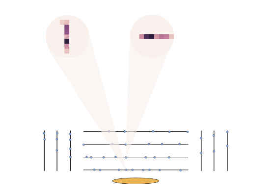
In the picture you can see a schematic view of the silicon tracker. The black lines represent the barrel and endcap layers, the orange part represents the interaction point, where the collision happened, and the blue circles represent the hit left by the particles on each layer, each one with its own shape.
We decided to deal with these differences using different feature maps for each layer. Our input image contains one channel for each layer, and they are all zero except for the correct layer. These representations allow us to train a single model for each configuration.
To represent the information about the crossing angle we also added some channels with angular corrections applied to the cluster shapes, to pass the angle information to our model.
Dataset Collection
The dataset is generated with a monte carlo simulation which generates particle trajectories simulating the LHC and the CMS detector, considering the magnetic field generated by the solenoid, the material budget, broken sensors and other types of interferences. The software used to generate the data is the CMSSW, available on github, which we modified to collect our dataset.
We extracted the doublets generated during the track reconstruction, along with several features for both the inner and outer hits:
- cluster shape
- global coordinates
- module and layer ID
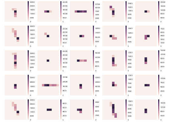
cluster shape samples extracted from the dataset.
We can notice many different patterns, corresponding to different particles or different directions.
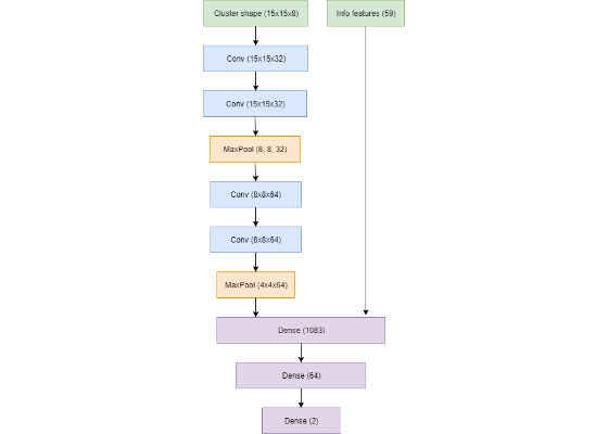
Model Architecture
Our proposed model is a convolutional neural network.
The choice of this model is determined by two main reasons. First, convolutional neural networks are a natural way to handle images, and they have been successful in computer vision tasks such as image classification, object recognition, and image segmentation, and in particle physics for event reconstruction (e.g. the NOvA experiment). Our problem is similar but the fundamental difference is that we need a smaller and faster model to run in real time. The second motivation is that neural network can easily run on GPU, and these help them scale up to large datasets. In the future, at least part of the track reconstruction will be executed entirely on GPU architectures.
This is the final architecture that we used:
Results
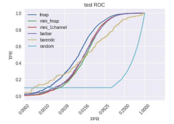
After training we tested our architecture on held-out data and we computed the ROC curve for different models.
- fmap is the model where each layer has a separated channel in the input shape
- mini_fmap is the fmap model with smaller parameters and a 7×7 shape instead of the standard 15×15
- mini_1channel is the mini_fmap without the layer separation in the input shape
- barbar is trained only with barrel-barrel data
- barendc is trained only with barrel-endcap data
- random is the ROC curve of the random model
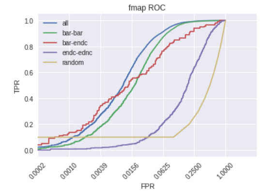
The ROC curves are plotted with a logarithmic scale on the x-axis because we are mainly interested in high levels of filtering. For the fmap model we also plotted the curve for different doublet modes.
Two main points can be noticed from these plots:
- we can filter about 75% of the data while keeping an efficiency (TPR) above 99%
- the performance for endcap-endcap is much lower than the other cases
We can effectively use this model to filter fake doublets but we must take some care. The problem with the endcap-endcap mode is that the data for this configuration is much less than the other two configurations. Probably a bigger dataset or rebalancing the dataset could solve the problem.
The next post will be about the computational cost at inference time for neural networks and how we can reduce it using different hardware or different models. I will also talk about weight quantization, binarized neural networks, and FPGA implementations for neural networks.
For more such intel IoT resources and tools from Intel, please visit the Intel® Developer Zone
Source:https://software.intel.com/en-us/blogs/2017/08/24/track-reconstruction-with-deep-learning-at-the-cern-cms-experiment