Fluid Simulation for Video Games (part 19)
")
From Vorticity through Vector Potential to Velocity
This and the next article in this series describe how to improve fidelity while reducing computational cost by combining techniques described in earlier articles. Fluid simulation entails computing flow velocity everywhere in the fluid domain. Most articles in this series advocate tracking vorticity (the curl of velocity), which describes how a flow rotates. So, the simulation must map vorticity into velocity.
Part 3 and part 4described how to do that by using an integral technique; part 6 described a differential technique. The integral technique has computational complexity O(N log N) and memory complexity O(N), whereas the differential technique has computational complexity O(N) and memory complexity O(N log N). When computers tend to have more abundant memory than computing power, the latter seems more attractive.
The differential technique (solving a vector Poisson equation) had another problem, however: boundary conditions. To solve a partial differential equation, you effectively already need a solution at the boundaries, which seems to have a circular dependency: To solve the equation, you need a solution.
In part 6, I dodged this problem by assuming a solution at the boundaries, then keeping the boundaries far from the region of interest. Unfortunately, this solution greatly expanded the domain size. Done the obvious way, that would consume more computing power and memory. If the domain increased by 3 times in each direction, memory and computing power would increase by 33 = 27 times. Instead, I decreased spatial resolution and held memory and computing power constant, so the overall result was that the differential method had lower fidelity.
There is another solution, however: Compute the solution at the boundaries using an integral technique. Remember, part 3 and part 4 explained how to integrate vorticity to get velocity, so you’re already familiar with an integral technique. In this case, I want to integrate vorticity to get the vector potential, not velocity. Fortunately, the technique for computing vector potential from vorticity also applies to computing velocity from vorticity: It simply uses a different formula for the integrand.
This article explains how to use O(N2) and O(N log N) integral techniques to compute vector potential, then reuses the approach from part 6 to compute velocity from vector potential. Figure 2 provides a comparison of these techniques. The subsequent article will apply the technique from this article to impose boundary conditions to solve the vector Poisson equation using the O(N) multigrid algorithm, yielding a faster algorithm with better fidelity than any of the algorithms presented so far in this series.

Figure 2: Comparison of fluid simulation techniques.
Part 1 and part 2 summarized fluid dynamics and simulation techniques. Part 3 and part 4 presented a vortex-particle fluid simulation with two-way fluid–body interactions that run in real time. Part 5 profiled and optimized that simulation code. Part 6 described a differential method for computing velocity from vorticity. Figure 1 shows the relationships between the various techniques and articles. Part 7 showed how to integrate a fluid simulation into a typical particle system. Part 8, part 9, part 10, and part 11 explained how to simulate density, buoyancy, heat, and combustion in a vortex-based fluid simulation. Part 12 explained how improper sampling caused unwanted jerky motion and showed how to mitigate it. Part 13 added convex polytopes and lift-like forces. Part 14, part 15, part 16, part 17, and part 18 added containers, smoothed particle hydrodynamics, liquids, and fluid surfaces.
Vector Potential
Recall from part 6 that the Helmholtz theorem states that a vector function ν can be decomposed into an irrotational part (∇φ) that has only divergence and a solenoidal part (∇ × A) that has only curl:

where:

Compare (2) with the formula from part 2 for obtaining velocity from vorticity ω, where ω = ∇ × v, using the Biot-Savart law:

Equation (3) formed the basis for the algorithm presented in part 3, which has been used throughout most of the articles in this series.
Notice that the integrals in equations (2) and (3) vaguely resemble each other. Numerical integration techniques used to compute velocity (v in equation (3)) also apply to vector potential (A in equation (2)). So, you can numerically integrate the vector potential A, then take the curl of A to get velocity: v=∇×A.
This approach might seem odd: Why bother going through the extra step of computing vector potential from vorticity, then taking its curl if you can directly compute velocity from vorticity? Because computing Aby solving a Poisson equation (∇2A=-ω) can be much faster within a domain interior, but you need to knowA on the domain boundaries. So, you can integrate vorticity to compute A on the domain boundaries, then solve a Poisson equation to compute A in the domain interior. That’s a lot of steps. So, this article focuses only on computing A everywhere by using the integral (2), then the next article will combine integral and differential techniques into a coherent solution.
What Is Vector Potential?
I find it useful to develop an intuition for quantities like velocity, vorticity, and vector potential. Figure 1 shows those quantities as vector fields. Most people have a sense for what velocity means: the direction and speed something moves. Vorticity is less familiar but still accessible: It’s like the axis about which some fluid rotates, where the axis points away from the clockwise face, and its length indicates how fast the fluid spins. Vector potential is a bit more abstract, but in Figure 1, vector potential looks like a diffused or blurred version of vorticity. That’s a clue for how to think about it.
The interpretation of vector potential as “diffused vorticity” dovetails well with Poisson’s equation. Consider an analogy to a block of metal heated or cooled at a collection of points. For example, it could be held at a higher temperature at one end and at a lower temperature at the opposite end. Given enough time, the heat will conduct through the block, and its temperature distribution will reach a steady state. The scalar version of Poisson’s equation describes the distribution of heat throughout the block.
With that mental model in mind, look at Figure 1 again. Imagine that vorticity is a heat source inside a block of metal suspended within a cooler environment. (In Figure 1, that heat source would be a ring, like the outer ring of a stove burner.) The vector potential looks something like what the temperature would be throughout that block: warm where red and cool where blue. One obvious difference here is that vorticity and vector potential are vectors, not scalars (like heat and temperature), but if you consider each component (x, y, and z) separately, each is a scalar field. (The x-component of vorticity is the “heat source” for the x-component of the vector potential “temperature” and so on for y and z.) So, the vector Poisson’s equation is almost like it describes three “flavors” of heat that propagate separately.
Computing Vector Potential by Integrating Vorticity
Analogous to the approach in part 3, you could replace the integral in equation (2) with a summation:

The summand in (4) has the problem that as ri becomes small (that is, as the query point x gets close to a vorton center), the 1/ri term becomes large. Using the same approach as in part 3, mollify the vortex by giving it a finite size. The summation then becomes:

The following macro implements the formula of equation (5):
#define VORTON_ACCUMULATE_VECTOR_POTENTIAL_private( vVecPot , vPosQuery , mPosition , mAngularVelocity , mSize , mSpreadingRangeFactor , mSpreadingCirculationFactor ) \
{ \
const Vec3 vOtherToSelf = vPosQuery – mPosition ; \
const float radius = mSize * 0.5f * mSpreadingRangeFactor ; \
const float radius2 = radius * radius ; \
const float dist2 = vOtherToSelf.Mag2() ; \
const float distLaw = ( dist2 < radius2 ) ? ( dist2 / ( radius2 * radius ) ) : ( finvsqrtf( dist2 ) ) ; \
const Vec3 vecPotContribution = TwoThirds * radius2 * radius * mAngularVelocity * distLaw ; \
vVecPot += vecPotContribution * mSpreadingCirculationFactor ; \
}
Note: See the archive file associated with this article for the rest of the code. Also, see part 3 for elaboration of these code snippets.
Direct Summation
You can use equation (5) by directly summing it for all vortons, for all query points. Assuming that you want to query at each vorton, that makes direct summation have asymptotic time complexity O(N2). The treecode presented below runs faster but makes some approximations. You can use the direct summation algorithm to compare other methods:
Vec3 VortonSim::ComputeVectorPotential_Direct( const Vec3 & vPosition )
{
const size_t numVortons = mVortons->Size() ;
Vec3 vecPotAccumulator( 0.0f , 0.0f , 0.0f ) ;
for( unsigned iVorton = 0 ; iVorton < numVortons ; ++ iVorton )
{ // For each vorton…
const Vorton & rVorton = (*mVortons)[ iVorton ] ;
VORTON_ACCUMULATE_VECTOR_POTENTIAL( vecPotAccumulator , vPosition , rVorton ) ;
}
return vecPotAccumulator ;
}
Treecode
The treecode algorithm for computing vector potential has identical structure to the treecode that computes velocity. It runs in O(N log N) time:
Vec3 VortonSim::ComputeVectorPotential_Tree( const Vec3 & vPosition , const unsigned indices[3] , size_t iLayer , const UniformGrid< VECTOR< unsigned > > & vortonIndicesGrid , const NestedGrid< Vorton > & influenceTree )
{
const UniformGrid< Vorton > & rChildLayer = influenceTree[ iLayer – 1 ] ;
unsigned clusterMinIndices[3] ;
const unsigned * pClusterDims = influenceTree.GetDecimations( iLayer ) ;
influenceTree.GetChildClusterMinCornerIndex( clusterMinIndices , pClusterDims , indices ) ;
const Vec3 & vGridMinCorner = rChildLayer.GetMinCorner() ;
const Vec3 vSpacing = rChildLayer.GetCellSpacing() ;
unsigned increment[3] ;
const unsigned & numXchild = rChildLayer.GetNumPoints( 0 ) ;
const unsigned numXYchild = numXchild * rChildLayer.GetNumPoints( 1 ) ;
Vec3 vecPotAccumulator( 0.0f , 0.0f , 0.0f ) ;
const float vortonRadius = (*mVortons)[ 0 ].GetRadius() ;
static const float marginFactor = 0.0001f ;
// When domain is 2D in XY plane, min.z==max.z so vPos.z test below would fail unless margin.z!=0.
const Vec3 margin = marginFactor * vSpacing + ( 0.0f == vSpacing.z ? Vec3(0,0,FLT_MIN) : Vec3(0,0,0) );
// For each cell of child layer in this grid cluster…
for( increment[2] = 0 ; increment[2] < pClusterDims[2] ; ++ increment[2] )
{
unsigned idxChild[3] ;
idxChild[2] = clusterMinIndices[2] + increment[2] ;
Vec3 vCellMinCorner , vCellMaxCorner ;
vCellMinCorner.z = vGridMinCorner.z + float( idxChild[2] ) * vSpacing.z ;
vCellMaxCorner.z = vGridMinCorner.z + float( idxChild[2] + 1 ) * vSpacing.z ;
const unsigned offsetZ = idxChild[2] * numXYchild ;
for( increment[1] = 0 ; increment[1] < pClusterDims[1] ; ++ increment[1] )
{
idxChild[1] = clusterMinIndices[1] + increment[1] ;
vCellMinCorner.y = vGridMinCorner.y + float( idxChild[1] ) * vSpacing.y ;
vCellMaxCorner.y = vGridMinCorner.y + float( idxChild[1] + 1 ) * vSpacing.y ;
const unsigned offsetYZ = idxChild[1] * numXchild + offsetZ ;
for( increment[0] = 0 ; increment[0] < pClusterDims[0] ; ++ increment[0] )
{
idxChild[0] = clusterMinIndices[0] + increment[0] ;
vCellMinCorner.x = vGridMinCorner.x + float( idxChild[0] ) * vSpacing.x ;
vCellMaxCorner.x = vGridMinCorner.x + float( idxChild[0] + 1 ) * vSpacing.x ;
if(
( iLayer > 1 )
&& ( vPosition.x >= vCellMinCorner.x – margin.x )
&& ( vPosition.y >= vCellMinCorner.y – margin.y )
&& ( vPosition.z >= vCellMinCorner.z – margin.z )
&& ( vPosition.x < vCellMaxCorner.x + margin.x )
&& ( vPosition.y < vCellMaxCorner.y + margin.y )
&& ( vPosition.z < vCellMaxCorner.z + margin.z )
)
{ // Test position is inside childCell and currentLayer > 0…
// Recurse child layer.
vecPotAccumulator += ComputeVectorPotential_Tree( vPosition , idxChild , iLayer – 1 , vortonIndicesGrid , influenceTree ) ;
}
else
{ // Test position is outside childCell, or reached leaf node.
// Compute velocity induced by cell at corner point x.
// Accumulate influence, storing in velocityAccumulator.
const unsigned offsetXYZ = idxChild[0] + offsetYZ ;
const Vorton & rVortonChild = rChildLayer[ offsetXYZ ] ;
if( 1 == iLayer )
{ // Reached base layer.
// Instead of using supervorton, use direct summation of original vortons.
// This only makes a difference when a leaf-layer grid cell contains multiple vortons.
const unsigned numVortonsInCell = vortonIndicesGrid[ offsetXYZ ].Size() ;
for( unsigned ivHere = 0 ; ivHere < numVortonsInCell ; ++ ivHere )
{ // For each vorton in this gridcell…
const unsigned & rVortIdxHere = vortonIndicesGrid[ offsetXYZ ][ ivHere ] ;
Vorton & rVortonHere = (*mVortons)[ rVortIdxHere ] ;
VORTON_ACCUMULATE_VECTOR_POTENTIAL( vecPotAccumulator , vPosition , rVortonHere ) ;
}
}
else
{ // Current layer is either…
// not a base layer, i.e. this layer is an "aggregation" layer of supervortons, …or…
// this is the base layer and USE_ORIGINAL_VORTONS_IN_BASE_LAYER is disabled.
VORTON_ACCUMULATE_VECTOR_POTENTIAL( vecPotAccumulator , vPosition , rVortonChild ) ;
}
}
}
}
}
return vecPotAccumulator ;
}
Parallelize Vector Potential Algorithms with Intel® Threading Building Blocks
You can use Intel® Threading Building Blocks (Intel® TBB) to parallelize either the direct summation or treecode algorithms. The approach follows that taken in part 3:
- Write a worker routine that operates on a slice of the problem.
- Write a wrapper functor class that wraps the worker routine.
- Write a wrapper routine that directs Intel TBB to call a functor.
Here is the worker routine
void VortonSim::ComputeVectorPotentialAtGridpoints_Slice( size_t izStart , size_t izEnd
, const UniformGrid< VECTOR< unsigned > > & vortonIndicesGrid , const NestedGrid< Vorton > & influenceTree )
{
const size_t numLayers = influenceTree.GetDepth() ;
UniformGrid< Vec3 > & vectorPotentialGrid = mVectorPotentialMultiGrid[ 0 ] ;
const Vec3 & vMinCorner = mVelGrid.GetMinCorner() ;
static const float nudge = 1.0f – 2.0f * FLT_EPSILON ;
const Vec3 vSpacing = mVelGrid.GetCellSpacing() * nudge ;
const unsigned dims[3] = { mVelGrid.GetNumPoints( 0 )
, mVelGrid.GetNumPoints( 1 )
, mVelGrid.GetNumPoints( 2 ) } ;
const unsigned numXY = dims[0] * dims[1] ;
unsigned idx[ 3 ] ;
for( idx[2] = static_cast< unsigned >( izStart ) ; idx[2] < izEnd ; ++ idx[2] )
{ // For subset of z index values…
Vec3 vPosition ;
// Compute the z-coordinate of the world-space position of this gridpoint.
vPosition.z = vMinCorner.z + float( idx[2] ) * vSpacing.z ;
// Precompute the z contribution to the offset into the velocity grid.
const unsigned offsetZ = idx[2] * numXY ;
for( idx[1] = 0 ; idx[1] < dims[1] ; ++ idx[1] )
{ // For every gridpoint along the y-axis…
// Compute the y-coordinate of the world-space position of this gridpoint.
vPosition.y = vMinCorner.y + float( idx[1] ) * vSpacing.y ;
// Precompute the y contribution to the offset into the velocity grid.
const unsigned offsetYZ = idx[1] * dims[0] + offsetZ ;
for( idx[0] = 0 ; idx[0] < dims[0] ; ++ idx[0] )
{ // For every gridpoint along the x-axis…
// Compute the x-coordinate of the world-space position of this gridpoint.
vPosition.x = vMinCorner.x + float( idx[0] ) * vSpacing.x ;
// Compute the offset into the velocity grid.
const unsigned offsetXYZ = idx[0] + offsetYZ ;
// Compute the fluid flow velocity at this gridpoint, due to all vortons.
static const unsigned zeros[3] = { 0 , 0 , 0 } ; // Starter indices for recursive algorithm
if( numLayers > 1 )
{
vectorPotentialGrid[ offsetXYZ ] = ComputeVectorPotential_Tree( vPosition , zeros , numLayers – 1
, vortonIndicesGrid , influenceTree ) ;
}
else
{
vectorPotentialGrid[ offsetXYZ ] = ComputeVectorPotential_Direct( vPosition ) ;
}
}
}
}
}
Here is the functor class:
class VortonSim_ComputeVectorPotentialAtGridpoints_TBB
{
VortonSim * mVortonSim ;
const UniformGrid< VECTOR< unsigned > > & mVortonIndicesGrid ;
const NestedGrid< Vorton > & mInfluenceTree ;
public:
void operator() ( const tbb::blocked_range<size_t> & r ) const
{ // Compute subset of vector potential grid.
SetFloatingPointControlWord( mMasterThreadFloatingPointControlWord ) ;
SetMmxControlStatusRegister( mMasterThreadMmxControlStatusRegister ) ;
mVortonSim->ComputeVectorPotentialAtGridpoints_Slice( r.begin() , r.end() , mVortonIndicesGrid , mInfluenceTree ) ;
}
VortonSim_ComputeVectorPotentialAtGridpoints_TBB( VortonSim * pVortonSim
, const UniformGrid< VECTOR< unsigned > > & vortonIndicesGrid
, const NestedGrid< Vorton > & influenceTree )
: mVortonSim( pVortonSim )
, mVortonIndicesGrid( vortonIndicesGrid )
, mInfluenceTree( influenceTree )
{
mMasterThreadFloatingPointControlWord = GetFloatingPointControlWord() ;
mMasterThreadMmxControlStatusRegister = GetMmxControlStatusRegister() ;
}
private:
WORD mMasterThreadFloatingPointControlWord ;
unsigned mMasterThreadMmxControlStatusRegister ;
} ;
Here is the wrapper routine:
void VortonSim::ComputeVectorPotentialFromVorticity_Integral( const UniformGrid< VECTOR< unsigned > > & vortonIndicesGrid
, const NestedGrid< Vorton > & influenceTree )
{
const unsigned numZ = mVelGrid.GetNumPoints( 2 ) ;
// Estimate grain size based on size of problem and number of processors.
const size_t grainSize = Max2( size_t( 1 ) , numZ / gNumberOfProcessors ) ;
// Compute velocity at gridpoints using multiple threads.
parallel_for( tbb::blocked_range<size_t>( 0 , numZ , grainSize )
, VortonSim_ComputeVectorPotentialAtGridpoints_TBB( this , vortonIndicesGrid , influenceTree ) ) ;
}
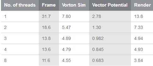
Performance
Table 1 shows the duration (in milliseconds per frame) of various routines, run on a 3.50‑GHz Intel® Core™ i7-3770K processor that has four physical cores and two local cores per physical core.
Table 1. The duration of various routines in milliseconds per frame.
Summary
This article applied the integral techniques presented in part 3 to compute the vector potential described in part 6. It’s meant as a stepping stone to a hybrid integral–differential technique: Part 20 in this series will describe how to use the differential technique (also presented in part 6) to compute for vector potential by solving a vector Poisson’s equation, where the boundary conditions will be specified using integral techniques. The hybrid solution will run faster and with better results than either the purely integral or purely differential technique alone.
Further Reading
Typically, I list references that I think elaborate on the topic, but in this unusual case, I could find little on the subject. I discovered one article in a Web search, although I admit that I have neither obtained nor read it. I choose to list it in case it helps any readers.
- Tutty, O.R. 1986. On vector potential-vorticity methods for incompressible flow problems. Journal of Computational Physics 64(2): 368-379.
About the Author
Dr. Michael J. Gourlay works at Microsoft as a principal development lead on HoloLens in the Environment Understanding group. He previously worked at Electronic Arts (EA Sports) as the software architect for the Football Sports Business Unit, as a senior lead engineer on Madden NFL*, and as an original architect of FranTk* (the engine behind Connected Careers mode). He worked on character physics and ANT* (the procedural animation system that EA Sports uses), on Mixed Martial Arts*, and as a lead programmer onNASCAR. He wrote Lynx* (the visual effects system used in EA games worldwide) and patented algorithms for interactive, high-bandwidth online applications.
He also developed curricula for and taught at the University of Central Florida, Florida Interactive Entertainment Academy, an interdisciplinary graduate program that teaches programmers, producers, and artists how to make video games and training simulations.
Prior to joining EA, he performed scientific research using computational fluid dynamics and the world’s largest massively parallel supercomputers. His previous research also includes nonlinear dynamics in quantum mechanical systems and atomic, molecular, and optical physics. Michael received his degrees in physics and philosophy from Georgia Tech and the University of Colorado at Boulder
For more such intel resources and tools from Intel on Game, please visit the Intel® Game Developer Zone
Source: https://software.intel.com/en-us/articles/fluid-simulation-for-video-games-part-19