Power System Infrastructure Monitoring Using Deep Learning on Intel Architecture

Abstract
 Survey
The work in this paper evaluates the performance of Intel® Xeon® processor powered machines for running deep learning on the GoogleNet* topology (Inception* v3). The functional problem tackled is the identification of power system components such as pylons, conductors, and insulators from the real-world video footage captured by unmanned aerial vehicles (UAVs) or commercially available drones. By conducting multiple experiments we tried to derive the optimal batch size, iteration count, and learning rate for the model to converge.
Introduction
Recent advances in computer-aided visual object recognition, namely the application of deep learning, has made it possible to solve a wide array of real-world problems which previously were impossible. In this work, we present a novel method for detecting the components of power system infrastructure such as pylons, conductor cables, and insulators.
The original implementation of this algorithm took advantage of the power of the NVIDIA* graphics processing unit (GPU) during training and detection. The current work primarily focuses on implementing the algorithm on TensorFlow* CPU mode and executing it over Intel® Xeon® processors.
During execution, we will record performance metrics across the different CPU configurations.
Environment Setup
Hardware Setup
Table 1. Intel® Xeon® processor configuration.
Software Setup
1. Python* Setup
The experiment is tested on Python* version 2.7.x. Verify the version as follows:
$ python –version
2. TensorFlow* Setup
1. Install TensorFlow using pip: “$ pip install tensorflow”. By default, this would install the latest wheel for your CPU architecture. Our experiment is built and tested on TensorFlow3 version 1.0.x.
2. Verify the installation using the command shown below:
$ python -c "import tensorflow; print(tensorflow.__version__)"
3. Inception* Model
The experiments detailed in the subsequent sections employ the transfer learning technique to speed up the entire process. For this purpose, we used a pretrained GoogleNet* model, namely Inception* v3. The details of the transfer learning process are explained in the subsequent sections.
Download the Inception v3 model from the following link: http://download.tensorflow.org/models/image/imagenet/inception-2015-12-05.tgz
4. TensorBoard*
We use TensorBoard* in our experiments to visualize the progress and the results of individual experiment runs.
TensorBoard is installed along with TensorFlow. After installing TensorFlow, enter the following command from the bash script to ensure that TensorBoard is available:
“ $ tensorboard –help ”
Solution Design
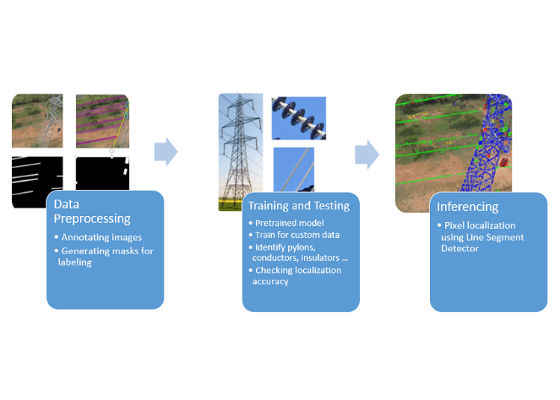
The entire solution is divided into three stages. They are:
- Data Preprocessing
- Model Training
- Inference
Figure 1. High-level solution design.
Data Preprocessing
The images used for training the model are collected through aerial drone missions carried out in the field. The images collected vary in resolution, aspect, and orientation, with respect to the object of interest.
The entire preprocessing pipeline is built using OpenCV* 2 (Python implementation). The high-level objective of preprocessing is to convert the raw, high-resolution drone images into a labeled set of image patches of size 32 x 32, which is used for training the deep learning model.
The various processes involved in the preprocessing pipeline are as follows:
- Image annotation
- Generating binary masks
- Creating labeled image patches
The individual processes involved in the pipeline are detailed in the following steps:
Step 1: Image annotation.
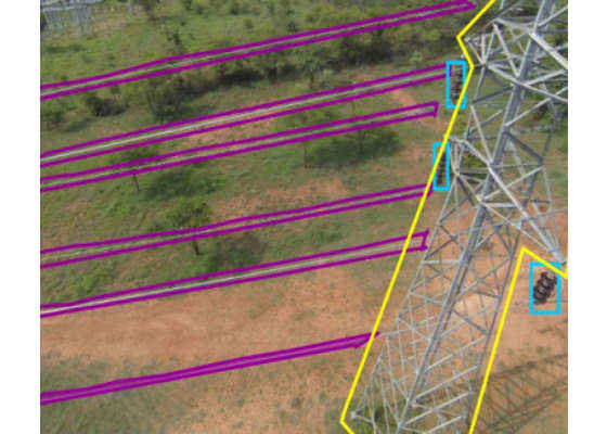
Those experienced in the art of building and training convolutional neural network (CNN) architectures will quickly relate to the image annotation task. It involves manually labeling the objects within your training image set. In our experiment, we relied on the Python tool, LabelImg*4, for annotation. The tool outputs the object coordinates in XML format for further processing.
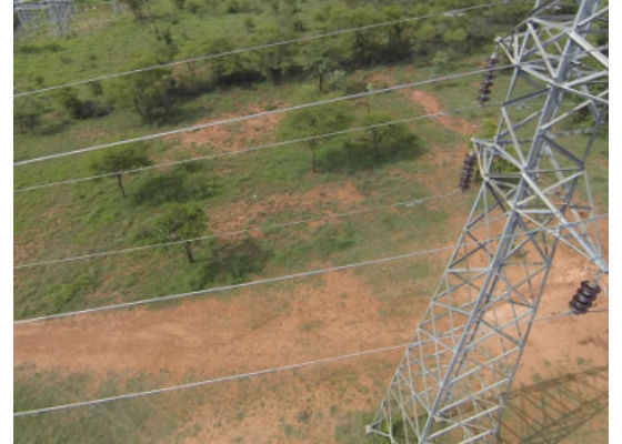
Figure 2. Image without annotation.
Figure 3. Image with annotation overlay.
The preceding images depict a typical annotation activity carried out on the raw images.
Step 2: Generating binary masks.
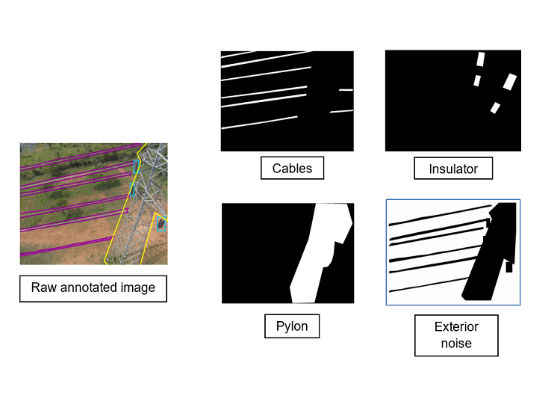
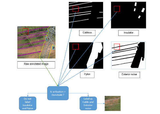
Binary masks refer to the mode of image representation where we depict either the presence or absence of an object. Hence, for every raw image, we generate individual binary masks corresponding to each of the labels available. The binary masks so created are used in the steps that follow for actually labeling the image patches. This idea is depicted in the following images. In the current implementation, the mask generation process is developed using Python OpenCV.
Figure 4. Generating binary masks from the raw image.
Step 3: Creating labeled image patches.
Once the binary mask is generated, we run a 32 x 32 filter over the raw image and compare the activations (white pixel count) obtained in the various masks for the corresponding filter position.
Figure 5. Creating labeled image patches.
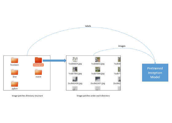
If the activation in a particular mask is found to be above the defined threshold of 5 percent of patch area (0.05*32*32), we label the patch to match the mask’s label. The output of this activity is a set of 32 x 32 image patches partitioned into multiple directories based on their labels. The forthcoming model training phase of the experiment directly accesses this partitioned directory structure for label-specific training images.
Figure 6. Preprocessing output directory structure.
Please note that in the above-described patch generation process, the total number of patches generated varies, depending on other variables such as size of the filter (32 x 32 in this case), resolution of input images, and the activation threshold, while comparing with binary masks.
Network Topology and Model Training
Inception v3 Model
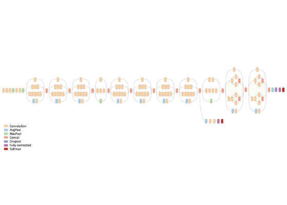
Figure 7. Inception V3 topology.
Inception V3 is a revolutionary deep learning architecture, which achieved state of the art performance in ILSVRC14 (ImageNet* Large Scale Visual Recognition Challenge 2014).
The most striking advantage of Inception over the other topologies is the depth of feature learning achieved, keeping the memory and CPU cost nearly at a par with other topologies. The architecture tries to improve on performance by reducing the effective sparsity of the data structures by converting them into dense matrices through clustering. This sparse-to-dense conversion is achieved architecturally by designing telescopic convolutions (1 x 1 to 3 x 3 to 5 x 5). This is commonly referred to as the network-in-network.
Transfer Learning on Inception
In our experiments we applied transfer learning on a pretrained Inception model (trained on ImageNet data). The transfer learning approach initializes the last fully connected layer with random weights (or zeroes), and when the system is trained for the new data (in our case, the power system infrastructure images), these weights are readjusted. The base concept of transfer learning is that the initial many layers in the topology will have learned some of the base features such as edges and curves, and this learning can be reused for the new problem with the new data. However, the final, fully connected layers would be fine-tuned for the very specific labels that it is trained for.
Hence, this needs to be retrained on the new data.
This is achieved through the Python API, as follows:
1. Add new hidden layer, Rectified Linear Unit (ReLU):
hidden_units_layer_1 = 1024
layer_weights_fc1 = tf.Variable(
tf.truncated_normal([BOTTLENECK_TENSOR_SIZE, hidden_units_layer_1], stddev=0.001),
name='fc1_weights')
layer_biases_fc1 = tf.Variable(tf.zeros([hidden_units_layer_1]), name='fc1_biases')
hidden_layer_1 = tf.nn.relu(tf.matmul(bottleneck_input, layer_weights_fc1,name='fc1_matmul') + layer_biases_fc1)
2. Add new softmax function:
layer_weights_fc2 = tf.Variable(
tf.truncated_normal([hidden_units_layer_1, class_count], stddev=0.001),
name='final_weights')
layer_biases_fc2 = tf.Variable(tf.zeros([class_count]), name='final_biases')
logits = tf.matmul(hidden_layer_1, layer_weights_fc2,
name='final_matmul') + layer_biases_fc2
final_tensor = tf.nn.softmax(logits, name=final_tensor_name)
Testing and Inference
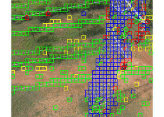
Testing is done on a 90:10 split on the entire image set. The test images go through the same patch generation process that was invoked during the training phase. The resultant patches are sent for detection on the trained model.
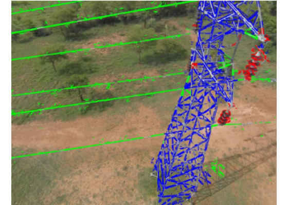
Figure 8. Result of model inference overlaid on raw image.
After detection, the patches are passed through a line segment detector (LSD) for the final localization.
Figure 9. Result of running LSD.
Results
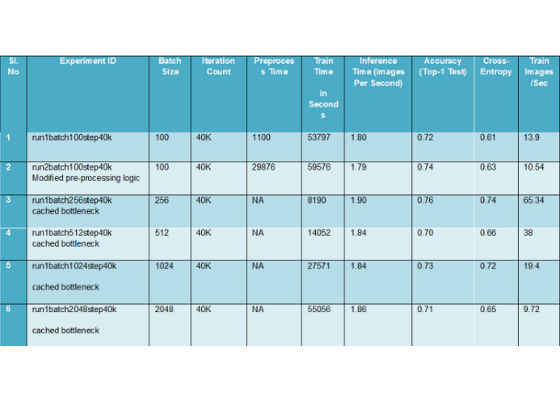
The different iterations of the experiments involve varying batch sizes and iteration counts.
During the experiments, in order to reduce the time consumed during preprocessing, we modified the preprocessing logic. Therefore, the metrics for different variants of the preprocessing logic were also captured.
We also observed that in the inception model, bottleneck tensors are cached during the initial run, so the training time during the subsequent runs would be much less. The final training result for the Intel Xeon processor is as follows:
Table 2. Experiment results.
Note: Inference time is inclusive of the preprocessing (patch) operation along with the time for the actual detection on the trained model.
Conclusion and Future Work
The functional use case tackled in this paper involved the detection and localization of power system components. The use case could be further expanded to identifying powersystem components that are damaged.
The training and inference time observed could be further improved by using an Intel optimized version of TensorFlow5.
List of Abbreviations
For more such intel IoT resources and tools from Intel, please visit the Intel® Developer Zone
Source:https://software.intel.com/en-us/articles/power-system-infrastructure-monitoring-using-deep-learning-on-intel-architecture

